Women Clothing Reviews

Background

Product reviews are very important for a company, as most consumers read reviews online before purchasing a product, they trust it as much as personal recommendations, and most reviews are expressive and honest. Product reviews also give companies ideas about how they can improve their products to increase customer’s satisfaction. In this post, I am going to predict how satisfied a consumer is after purchasing a product, based on their product reviews, specifically, the text reviews. The dataset is available at my Github.

Data exploration

Lets read the data and see what it looks like.

data = pd.read_csv('C:/Github/women_clothing/Womens_Clothing_Reviews.csv', header=0)
data = data.rename(columns={list(data)[0]: 'count'})
data.head(2)
print ('Column Name: '+ str(list(data)))

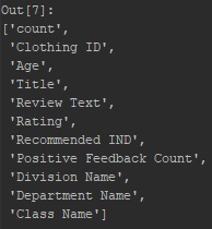
The data is loaded successfully. As we can see in the dataset, there are columns such as “Recommended IND” and “Positive Feedback Count” in the dataset. However, I am going to ignore them as this project focuses on text analysis. That being said, let’s explore how the text length has an influence on ratings.

Data Exploration

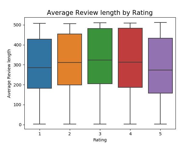
The trend of this boxplot looks like a mini pyramid, as the average text length increases and reaches it’s top at rating 3, then descends at the same rate and finally reaches rating 5. It means that purchasers who rated their products as 3 may have given more details in the reviews compared to the ones who rated 1 or 5.

Word cloud is a method that shows the most frequent words in a text. We often can find interesting insight as we can see the reasons why consumers rank their items in a certain ratings.

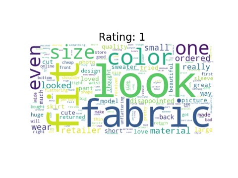
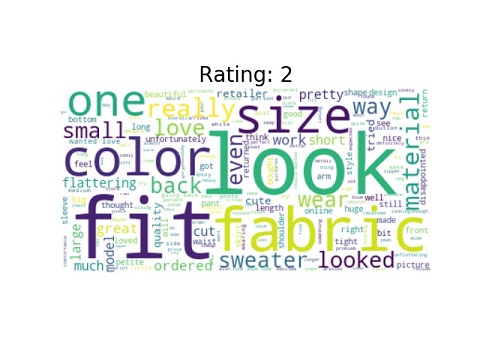
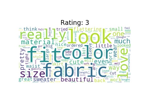
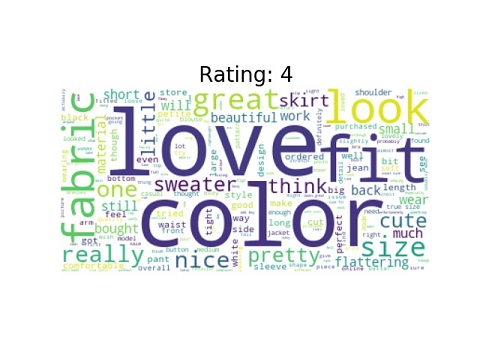
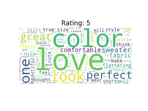
Some common words among all or most ratings are look, fabric, color, and fit. In Rating 1, there are negative words such as disappointed, small, and unflattering. Surprisingly, positive words can be seen in this cloud like great and cute. Starting from rating 3, we no longer see negative words in the cloud. More and More positive words start to dominate the cloud such as beautiful, pretty, and love. The number of positive words once again grow as rating reaches rating 5. In fact, love and perfect take over and eventually dominate the cloud.

Sentiment Analysis

Those clouds helped us visualize what consumers generally think when writing reviews. We can further translate these messages into numeric values by implementing sentiment analysis. I am using SentimentIntensityAnalyzer from NLTK in order to calculate the sentiment scores for each sentence. I am only using three of the outputs this function returned: neg, neu, and pos, which correspond to negative, neutral, and positive. For each text review, The sum of these three values equals to one. For example, “This dress is absolutely perfect” will return (0.0, 0.5, 0.5), which means .5 in both neutral and positive.

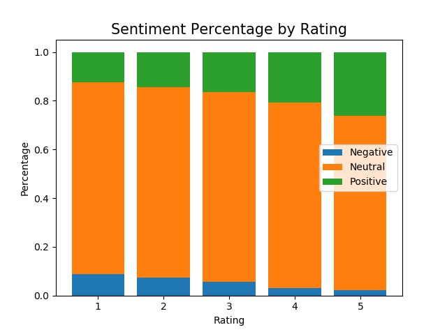
There are a couple of interesting insights from this bar chart.

• The percentage of negative emotion decreases as rating increases, while the percentage of positive emotion increases as rating increases.
• Neutral emotion is the major part of the reviews and it remains stable throughout all ratings.
• Positive percentages are greater than negative percentages across all ratings, even in rating 1.

Machine Learning Model

Text data requires additional modifications before passing it to the machine learning model:

• Tokenization: parsing each text into bags of words
• Vectorization: all words will be encoded into numbers to be passed to a machine learning model.

Sci-kit learn’s countVectorizer can separate text into tokens and count the frequency of each token. For example, consider a block of text: [ “This dress cute”, “I hate this dress”, “dress too small”]. It will return:

The first column corresponds to the text index. The second column and beyond are binary values of whether a particular word exists in that text.

There are a number of techniques I could use when applying CountVectorizer to the text. Applying these techniques can clean the text and simplify the machine learning model:

• Removing stopword and punctuations.
• Stopword means common words in English, e.g. the, her, this, etc.
• Stemming and lemmatization: techniques that are used to prepare text for further processing
• Stemming removes suffixes and prefixes such as -ed, -s, and -ize. Sometimes it may result in a word that is not an actual word. e.g. humble -> humbl
• Lemmatization makes sure the modified word is an actual word in English, but it is slower than stemming and need to define which part you want to modify.
• N-gram: a set of consecutive words. E.g. great dress, small sweater.
• Min_df/ Max_df: ignore words in which their frequency is lower/higher than a given threshold. An example of min_df would be a typo, and an example for max_df would be a common word like look and dress.

In addition to CountVectorizer, I also implement TD-IDF vectorizer to the text data. TD-IDF stands for term frequency - inverse document frequency, which vectorizes text by figuring out what terms are the most relevant for a document. For example, say there is a text review, “I hate this dress”. Since customers generally do not use negative words when writing reviews, it is reasonable to assume “hate” is much less frequent among all text reviews compared to the word like “this” or “dress”. In other words, this word must be more useful than the words like “this” and “dress”, and therefore “hate” will have a higher score compared to “this” or “dress”.

  stemmer = PorterStemmer()

  def clean_mess(text):
      step1 = [i for i in text if i not in string.punctuation]
      step2 = ''.join(step1)
      step3 = ' '.join([i for i in step2.split() if i.lower() not in sw])
      step4 = [stemmer.stem(i) for i in step3.split()]
      return step4

  vector = CountVectorizer(stop_words=sw, ngram_range=(1,3), min_df=9, analyzer=clean_mess)
  vector2 = TfidfTransformer()
  training = vector.fit_transform(data['Review Text'])
  training2 = vector2.fit_transform(training)

I am going to use Naïve Bayes as my machine learning algorithm. Naïve Bayes is a machine learning algorithm that is easy and fast to predict classes; however, it requires independence assumption. Even though it is impossible to consider all predictors are completely independent, It is still reasonable to make such an assumption as each review is independent than the others. The primary reason I am implementing this algorithm is that its computational requirement is minimal compared to other algorithms like random forest.

As usual, I split the data into a training set and test set in order to avoid overfitting. The dimension of the features are 17614 * 2826 and there are five possible outcomes: rating 1-5. I am going to use accuracy as my evaluation metric. The accuracy is calculated by the correct predictions over the all possible predictions. I set the benchmark to be 20% since there is a 20% chance of getting the correct answer randomly. If the machine learning model predicts higher than 20%, then we can conclude that the text is helpful in predicting customer ratings.

It turns out the accuracy is 60%, which is significantly higher than random guessing. It is possible to tune the model or to try different machine learning algorithms to see if we can get a better accuracy, but I will leave it as future improvements. This post has shown the potential for text analysis and how we can implement natural language processing techniques to get valuable information from customer reviews. This post on text mining definite helps the company know more about its customers, and more importantly, to know more about what customers care about in term of the online shopping experience.