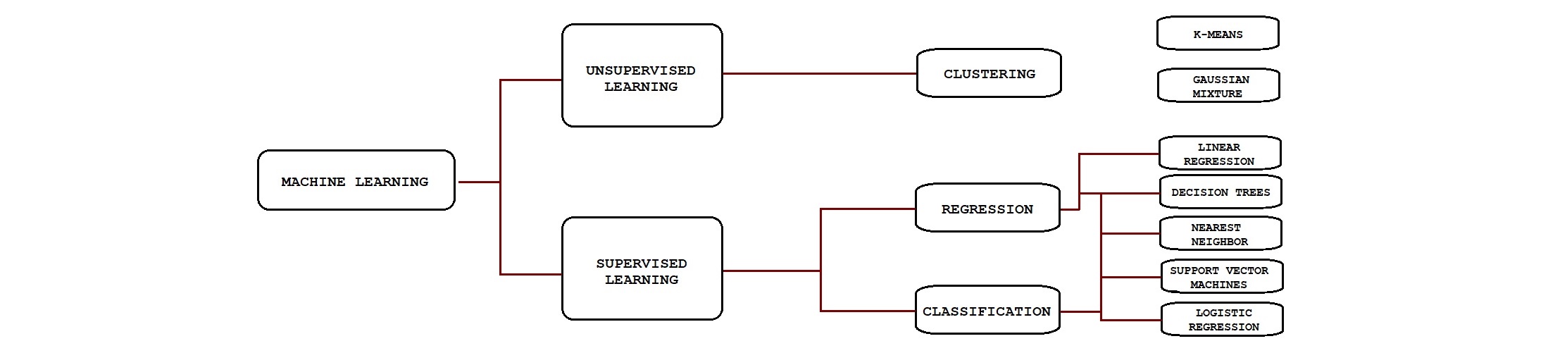
How do Machine Learning Algorithms work?

Logistic Regression

Logistic regression measures the relationship between the categorical dependent variable and one or more independent variables by estimating probabilities using a logistic function. (Wikipedia)

Characteristics of Logistic regression

• Widely used in many classification problems
• Output can be interpreted as probability
• Perform well even in a small dataset
• Cannot solve non-linear problem

How does logistic regression work?

Let’s consider a scenario in which we are predicting whether a person has diabetes based on their age and weight.

We first plug the predictors into a linear function: \(L=b_0+b_1 age+b_2 weight\). We called L as log-odds, which is a linear combination of age and weight, with \(b_0\) as a constant, and \(b_1, b_2\) as coefficients. We then transform the log-odds to probabilities using the logistic regression formula: \(p=\frac{e^L}{1+e^L}\).

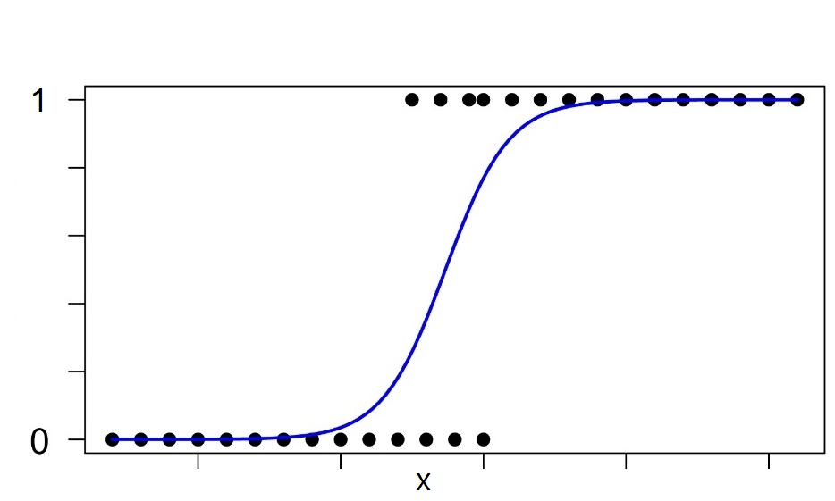
This formula gives us a S-shaped probability distribution, with the range 0 to 1. Therefore, we can interpret \(p\) as probability. We then apply log to all data points after plugging into the formula above. Adding them up gives us their likelihood of that particular S-shaped function. The best model can be achieved when we maximize the likelihood. In order to accomplish the maximum likelihood, we keep rotating the log odds line and repeat the calculation above.

Therefore, logistic regression is more like a linear classifier where it calculates a score (probability) to predict whether it belongs to 0 or 1.

Decision Trees

Decision trees breakdown a dataset into smaller subsets (decision nodes, chance nodes, and end nodes). Decision nodes indicate a decision to be made, and chance nodes are the children of decision nodes, which shows the probability of certain results. End nodes represent the outcome of the model. Decision trees are built using a technique called ID3, which use entropy and information gain to construct a decision tree.

Definition

Before we explore how decision trees works, we need to understand the following terms:

• Purity: how well two (or more) classes are separated after the split.
• Entropy: It indicates how pure one subset is. In other words, it tells you how un-certain you are about a randomly picked item is yes or no. We want to minimize entropy as much as possible. We will explore further below in detail.
• Information gain: It measures how useful a feature is for splitting the label (yes/no). We want to maximize information gain, and the feature with the highest information gain will split first.

Characteristics of Decision Trees

• Easy to understand and explain
• Can handle non-linear features
• Prone to overfitting
• cannot train unseen categorical values

How does Decision Trees work?

There are many ways to measure the purity of the split. One way is utilizing entropy and information gain. Entropy: \(H(S) = -p_1 log_2 p_1 – p_0 log_2 p_0\), where \(S\) is the subset of training examples, \(p_1\) is the percentage of positive examples in \(S\), \(p_0\) is the percentage of negative examples in \(S\).

Entropy

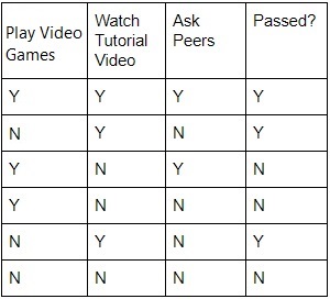
Consider the table above, if we do NOT ask peers, there will be 4 possible outcomes: 2 Yes (indicating pass) and 2 No (indicating no pass). The entropy, \(H(S)\), then would be \(-0.5 log_2 0.5-0.5 log_2 0.5=1\) bit. On the other hand, if we watch video, we will be have 3 possible outcomes, which are all yes. \(H(S)\) would be \(1 log_2 1 - 0 log_2 0=0\) bit.

Information gain

The equation of information gain is \(Gain(S,A)=H(S)-\sum_{v\in values(A)}[\frac{\|S_v\|}{\|S\|}H(S_v)]\), where A is an predictor, v is the value of the predictor.

let A = playing video games, and B = not playing video games. The information gain of playing games is: \(Gain(S, game)= H(S) - ( p(A)H(S_A)+p(B)H(S_B) )\). Here \(H(S) = 1\) because there are 6 possible outcomes, 3 yes and 3 no. The probability of playing games is 3/6, and the probability of not playing games is \(\frac{3}{6}\).

The entropy of playing games is \(-0.33 log_2 0.33-0.67 log_2 0.67=0.91\), and entropy for not playing games is \(-0.67 log_2 0.67-0.33 log_2 0.33=0.91\).

Therefore, \(Gain(S, "game")= 1 - ( 0.5*0.91+0.5*0.91 )=0.09\) \(Gain(S, "video")= 1 - ( 1*0+0*0 )=1\) \(Gain(S, "Ask peers")= 1 - ( \frac{2}{6} * 1 + \frac{4}{6} * 1 )=0\)

Since we are trying to maximum the information gain, the predictor we split first for predicting whether we are going to pass or not is watching tutorial videos (yes/no).

Naïve Bayes

Naïve Bayes is a simple yet powerful machine learning algorithm that does a great job in supervised learning. It uses a probability theory, Bayes’ theorem, to make classifications.

Characteristics of Naïve Bayes

• generally useful in NLP (text) problems
• Easy and fast to make predictions
• performs well in multi-class predictions
• Assuming each feature is independence of one another
• Performs well when inputs are categorical variables
• If a variable in the test set has a new value that is never observed in the training phrase, it will return 0 probability (although can be solved with some techniques)

How does Naïve Bayes work?

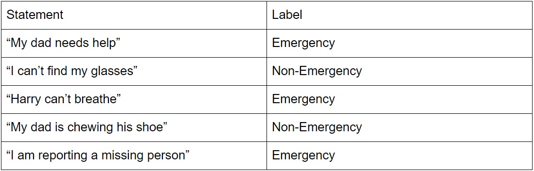
Consider the table above, if we have a new statement “Help my dad is missing”, how does Naïve Bayes decide whether it is emergency or non-emergency statement?

Word frequencies. Based on how many times a word occurs in a sentence, given its label, we can get a sense of how it belongs to one label or not using Bayes Theorem: \(P(A\|B)= \frac{P(B\|A)P(A)}{P(B)}\).

Let’s say A is an Emergency statement, and B is the text sentence we are interested in testing. By assuming each word is independent of one another, P(help my son is missing) = \(P(help) * P(my) * P(son) * P(is) * P(missing)\), where \(P\) indicates probability.

We now have every info to calculate the probability for this problem; starting with \(P(A)\), the probability of an emergency statement, appeared three out of five times, therefore \(P(A)=\frac{3}{5}\).

\(P(help)\) is the frequency of help out of all word frequency: \(\frac{1}{4+5+3+6+6} = \frac{1}{24}\), \(P(my) = \frac{2}{24}\), \(P(dad) = \frac{2}{24}\), \(P(is) = \frac{1}{24}\), \(P(missing) = \frac{1}{24}\).

P(help|Emergency) means the probability of the frequency of “help” appeared in Emergency label: \(P(help\|Emergency)=\frac{1}{13}\), \(P(my\|Emergency) = \frac{1}{13}\), \(P(dad\|Emergency) = \frac{1}{13}\), \(P(is\|Emergency) = \frac{0}{13}\), \(P(missing) = \frac{1}{13}\).

Then the equation becomes:

P(Emergency|“help my dad is missing”) = \(\frac{P(help\|Emergency)P(my\|Emergency)P(dad\|Emergency)P(is\|Emergency)P(missing\|Emergency)P(Emergency)} {P(help)P(my)P(dad)P(is)P(missing)}\)

Note that P(is|Emergency) = 0, which will mess up the calculation as everything multiple by 0 is 0. To solve this issue, we need to apply Laplace smoothing, which add all unique words by 1. That is, to add 19 to the denominator, and add 1 to the numerator. E.g. \(P(help\|Emergency) = \frac{2}{32}\).

Then the equation becomes: P(Emergency|“help my dad is missing”) = \(\frac{(\frac{2}{32}* \frac{2}{32} * \frac{2}{32} * \frac{1}{32} * \frac{2}{32})(\frac{3}{5})} {\frac{2}{43} * \frac{3}{43} * \frac{3}{43} * \frac{2}{43} * \frac{3}{43} } = 0.389\)

P(Non-Emergency|“help my dad is missing”) = \(\frac{(\frac{1}{32} * \frac{3}{32} * \frac{2}{32} * \frac{2}{32} * \frac{1}{32})(\frac{2}{5})}{(\frac{2}{43} * \frac{3}{43} * \frac{3}{43} * \frac{2}{43} * \frac{3}{43})} = 0.173\)

As a result, the probability of being an emergency statement is 0.389, and being an non-emergency statement is 0.173. In addition, the likelihood of the event, or likelihood of being an emergency statement , is \(\frac{0.389}{(0.389+0.173)} = .692\). Since 0.692 is higher than 0.5, the model will label this sentence as emergency statement.

Support Vector Machine

What is support vector machine?

support vector machine is an algorithm that can be used for regression and classification. It applies kernel trick to transform data in order to find the best way to separate classes.

Characteristics of Support Vector Machine

• Can handle non-linear features
• Great at dealing with high dimensional data
• Hard to interpret when the transformations become complex
• Slow training time for large dataset
• bad performance when many noises exist/ overlapping classes.

How does Support Vector Machine work?

(give an graphic example) The goal of SVM is to choose a line, or hyperplane, that has the widest margin that separates two or more classes. In other words, we want a hyperplane that leaves as much space as possible between two classes. Kernel trick: Kernel trick is one of the most important elements in SVM. it transform and combine predictors in order to create a new dimension that can linearly separate two or more classes.

SVM model parameters: C: prevent overfitting; allows you to decide how much you want to penalize misclassified points; higher C means heavier penalties on misclassification. Kernel: linear, rbf, polynomial, sigmoid Rbf requires a new parameter called gamma, large gamma means more complexity (easy to overfit).